Overview

This guide is meant to give you an overview of all the important parts of FactorioCalc. It does not spell out all the details for every function introduced and assumes the examples provided are sufficient. For complete documentation see the API docs. A decent knowledge of how to play Factorio is assumed.

This guide is also available as a Jupyter notebook for use in Google Colaboratory or your own Jupyter instance. A older version of this guide (0.2.0) is also available with JupyterLite so that you can try the examples yourself.

Basics

To use FactorioCalc you need to import it and call setGameConfig to set the game configuration to match the version of Factorio you are using. This section of the guide will assume you are using Factorio 2.0 without the Space Age addons.

All symbols you need are exported into the main factoriocalc namespace so it is rare you will need to import from a sub-module. FactorioCalc is meant to be used interactively via a REPL, with details of your overall factory collected in a simple script, or in a Jupyter notebook. For this reason it is acceptable to use from factoricalc import * and the rest of the documentation will assume you have done so.

from factoriocalc import *
setGameConfig('v2.0');

For lack of a better term, factory, will be used throughout this document to refer to any group of machines that work together to produce one or more products. The term overall factory will be used to refer to all the factories on the map.

Factoricalc uses exact fractions internally. For speed a custom fraction class is used. This class does not allow conversion from floats, as 0.12 as a float is not 12/100 but really 1080863910568919/9007199254740992, which is almost certainly not what was intended. There are various heuristics that can be used to give a better conversion, but for now it is easier to disallow them. In almost any place that expects a number a string can be used instead, in the rare case a number is needed the frac() function can be used to create a Frac. For example: frac('0.12'), frac('1/3'), frac(1,3).

Each machine is a class in the runtime generated mch package. The name of the machine is the same as the internal name but converted to TitleCase. The internal name is often the same as the English name, but not always. To find a machine based on the translated name you can use the mch._find() function. To get the translated name of a machine use the descr property.

To produce something from a machine you need to instantiate it. The first argument of the constructor is the recipe. For example, to create an “assembling-machine-3” that produces electronic circuits you could use mch.AssemblingMachine3(rcp.electronic_circuit). Additional keyword arguments can be provided to specify the fuel used, beacons, and modules, when applicable.

Recipes are in the runtime generated rcp package and are the same as the internal names but with - (dashes) converted to _ (underscores). Items are in itm. Like the mch package, both the rcp and itm package have have a _find() function to find an item based on the translated name.

Within FactorioCalc the items a machine produces or consumes is considered a flow. The rate of the flow is positive for items produced and negative for items consumed.

To get the flow of items for a machine use the flows() method, for example:

mch.AssemblingMachine3(rcp.electronic_circuit).flows()

<<iron_plate -2.5/s> <copper_cable -7.5/s> <electronic_circuit 2.5/s> <electricity -0.3875 MW>>

(Note that electricity used is also tracked as a flow.) To get a nicer formatted version of the flows, use the print() method:

mch.AssemblingMachine3(rcp.electronic_circuit).flows().print()

  iron_plate -2.5/s
  copper_cable -7.5/s
  electronic_circuit 2.5/s
  electricity -0.3875 MW

Multiple machines can be grouped together using the + operator which will create a Group. For example:

ec = mch.AssemblingMachine3(rcp.electronic_circuit) + mch.AssemblingMachine3(rcp.copper_cable)
ec

Group(mch.AssemblingMachine3(rcp.electronic_circuit), mch.AssemblingMachine3(rcp.copper_cable))

We can then get the flows of the group using the flows() method:

ec.flows().print()

  electronic_circuit 2.5/s
  copper_cable! -2.5/s (5/s - 7.5/s)
  iron_plate -2.5/s
  copper_plate -2.5/s
  electricity -0.775 MW

This is showing us the maximum rates for the group, but there is a problem: we are creating copper cables at a rate of 5/s but consuming them at -7.5/s. The ! after copper cables indicates a lack of an ingredient. We can fix this by using the correct ratios or by slowing down the machine that creates electronic circuits by adjusting it’s throttle.

To fix the ratios we can use the * operator to create multiple identical machines. For example:

ec2 = 2*mch.AssemblingMachine3(rcp.electronic_circuit) + 3*mch.AssemblingMachine3(rcp.copper_cable)

If we ask for the flows of the new Group we get:

ec2.flows().print()

  electronic_circuit 5/s
  copper_cable 0/s (15/s - 15/s)
  iron_plate -5/s
  copper_plate -7.5/s
  electricity -1.9375 MW

To instead slow down the machines we need to adjust the throttle. We can do this manually, but it’s best to let the solver determine it for us. To do so, we first need to wrap the group in a box:

b = Box(ec)

and then solve it:

b.solve()

<SolveRes.UNIQUE: 2>

The result of solve tells us a single unique solution was found. If we ask for the flows of the solved box we get:

b.flows().print()

  electronic_circuit 1.66667/s
  iron_plate -1.66667/s
  copper_plate -2.5/s
  electricity -0.65 MW

Copper-cable is not in the list because it’s net flow is now zero. Boxes, unlike groups, do not include internal flows unless the net flow is non-zero. An internal flow is simply a flow in which there are both producers and consumers within the same box.

As creating a box and then solving it is a very common operation the box shortcut function is provided to do just that, it usage is the same as the Box constructor. For example, we could of instead used:

b = box(ec)

To determine what the solver did we can use the summary() method. Calling it gives us:

b.summary()

b-electronic-circuit:
       1x electronic_circuit: AssemblingMachine3  @0.666667
       1x copper_cable: AssemblingMachine3
  Outputs: electronic_circuit 1.66667/s
  Inputs: iron_plate -1.66667/s, copper_plate -2.5/s

The @0.66667 indicates that the assembling machine for the electronic-circuit is throttled and only running at 2/3 it’s capacity.

Modules And Beacons

Having to spell out the type of machine you want each time will get tedious very fast so FactorioCalc provides a shortcut. However, before we can use the shortcut, we need to specify what type of assembling machine we want to use. This is done by setting config.machinePrefs, which is a python ContextVar. For now we will set it to MP_LATE_GAME in the presets module which will use the most advanced machines possible for a recipe:

from factoriocalc.presets import *
config.machinePrefs.set(MP_LATE_GAME);

With that we can simply call a recipe to produce a machine that will use the given recipe. Now to create electronic circuits from copper and iron plates we can instead use:

ec2 = 2*rcp.electronic_circuit() + 3*rcp.copper_cable()

Of course in the late game we are going to want to use productivity-3 modules with beacons stuffed with speed-3 modules. We can either pass modules and beacons to the call above, or include them in the machinePrefs.

To include them in the call simply use the modules and beacons parameter. For example, to make electronic circuits with 4 productivity-3 modules and 8 beacons with speed-3 modules use:

rcp.electronic_circuit(modules=4*itm.productivity_module_3,
                       beacons=8*mch.Beacon(modules=2*itm.speed_module_3))

mch.AssemblingMachine3(rcp.electronic_circuit, modules=4*itm.productivity_module_3, beacons=8*mch.Beacon(2*itm.speed_module_3))

When specifying modules you can either provide a list of them (as above) or a single module to fill the machine to with as many of that module as possible. When you need a beacon with two speed-3 modules you can use the SPEED_BEACON shortcut in presets. For example, the above call can become:

rcp.electronic_circuit(modules=itm.productivity_module_3,
                       beacons=8*SPEED_BEACON)

mch.AssemblingMachine3(rcp.electronic_circuit, modules=4*itm.productivity_module_3, beacons=8*mch.Beacon(2*itm.speed_module_3))

Specifying the modules and beacons configuration for each machine can be tedious, so as an alternative FactorioCalc lets you set preferred machine configurations as part of config.machinePrefs. If all we cared about is assembling machines we could just use:

config.machinePrefs.set([mch.AssemblingMachine3(modules=itm.productivity_module_3, 
                                                beacons=8*SPEED_BEACON)]);

However, we will most likely want all the machines to have the maximum number of productivity-3 modules and at least some speed beacons. To make this easier the MP_MAX_PROD function can used to indicate that we want all machines to have to maximum number of productivity-3 modules. There is no preset for beacons, as the number the beacons often varies. Instead use the withBeacons() method to modify the preset by adding SPEED_BEACON’s for specific machines. For example:

config.machinePrefs.set(MP_MAX_PROD().withBeacons(SPEED_BEACON, {mch.AssemblingMachine3:8}));

will give all machines the maximum number of productivity-3 modules possible and all assembling-machine-3s 8 SPEED_BEACON’s. With machinePrefs set we can than just use:

rcp.electronic_circuit()

mch.AssemblingMachine3(rcp.electronic_circuit, modules=4*itm.productivity_module_3, beacons=8*mch.Beacon(2*itm.speed_module_3))

Now lets try and combine electronic circuits with copper cables with maximum productivity. We could calculate the exact ratios or just guess and let the solver do most of the math for use:

ec3 = box(rcp.electronic_circuit() + rcp.copper_cable())
ec3.summary(includeMachineFlows=True)

b-electronic-circuit:
       1x electronic_circuit: AssemblingMachine3  @0.933333  +364% speed +40% prod. +914% energy +40% pollution:
             electronic_circuit~ 15.1660/s, iron_plate~ -10.8328/s, copper_cable~ -32.4985/s, electricity -3.56139 MW
       1x copper_cable: AssemblingMachine3  +364% speed +40% prod. +914% energy +40% pollution:
             copper_cable 32.4985/s, copper_plate -11.6066/s, electricity -3.81489 MW
  Outputs: electronic_circuit 15.1660/s
  Inputs: iron_plate -10.8328/s, copper_plate -11.6066/s

(The includeMachineFlows parameter will include the flows of individual machine groups in the summary. The ~ after an item in the flows indicates the flow has been adjusted due to throttling.)

Looking at the above summary the electronic circuit are throttled at 93%, so a 1:1 ratio is fairly close. We could increase the number of machines, but given the high flow of items, doing so will likely be difficult. Maybe we can decrease the number of beacons for the electronic circuits:

ec3 = box(rcp.electronic_circuit(beacons=6*SPEED_BEACON) + rcp.copper_cable())
ec3.summary()

b-electronic-circuit:
       1x electronic_circuit: AssemblingMachine3  +307% speed +40% prod. +834% energy +40% pollution
       1x copper_cable: AssemblingMachine3  @0.940252  +364% speed +40% prod. +914% energy +40% pollution
  Outputs: electronic_circuit 14.2598/s
  Inputs: iron_plate -10.1856/s, copper_plate -10.9131/s

That is only slightly better, but instead of not producing enough copper cables we are producing more than enough, which is generally a better thing to do.

Using produce

Basic Usage

In the previous section we manually combined the machines. It is also possible to use the produce function to automatically determine the required machines. For example to produce electronic circuits at 30/s:

ec4 = produce([itm.electronic_circuit @ 30]).factory
ec4.summary()

b-electronic-circuit:
    1.85x electronic_circuit: AssemblingMachine3  +364% speed +40% prod. +914% energy +40% pollution
    40.8x iron_plate: ElectricFurnace  -30% speed +20% prod. +160% energy +20% pollution
    1.98x copper_cable: AssemblingMachine3  +364% speed +40% prod. +914% energy +40% pollution
    43.7x copper_plate: ElectricFurnace  -30% speed +20% prod. +160% energy +20% pollution
  Outputs: electronic_circuit 30/s
  Inputs: iron_ore -17.8571/s, copper_ore -19.1327/s

The @ operator pairs an item with a rate and returns a tuple. The .factory at the end of produce is necessary because produce returns a class with additional information about the solution it found, but for now we only are interested in the result.

And, oops, we forgot to include speed beacons for electric furnaces in the previous section. I personally don’t find it worth it to use modules for basic smelting even in the late game so instead let’s just change machinePrefs to that effect:

config.machinePrefs.set([mch.ElectricFurnace(),
                        *MP_MAX_PROD().withBeacons(SPEED_BEACON, ({mch.AssemblingMachine3:8}))])
ec4 = produce([itm.electronic_circuit @ 30]).factory
ec4.summary()

b-electronic-circuit:
    1.85x electronic_circuit: AssemblingMachine3  +364% speed +40% prod. +914% energy +40% pollution
    34.3x iron_plate: ElectricFurnace
    1.98x copper_cable: AssemblingMachine3  +364% speed +40% prod. +914% energy +40% pollution
    36.7x copper_plate: ElectricFurnace
  Outputs: electronic_circuit 30/s
  Inputs: iron_ore -21.4286/s, copper_ore -22.9592/s

Ok, we still need a lot of electronic furnaces, but I normally smelt in a separate factory. So let’s instead create electronic circuits from just iron and copper plates by using the using keyword argument:

ec5 = produce([itm.electronic_circuit @ 30], using = [itm.iron_plate, itm.copper_plate]).factory
ec5.summary()

b-electronic-circuit:
    1.85x electronic_circuit: AssemblingMachine3  +364% speed +40% prod. +914% energy +40% pollution
    1.98x copper_cable: AssemblingMachine3  +364% speed +40% prod. +914% energy +40% pollution
  Outputs: electronic_circuit 30/s
  Inputs: iron_plate -21.4286/s, copper_plate -22.9592/s

The using keyword argument is a list that guides the machine selection process: if the element is an item produce will attempt to use that item and then stop once it does, if the element is a recipe than produce will prefer that recipe over another when there are multiple possibles.

Inputs can also be paired with a rate to use up to that amount of items. When rates are specified for the inputs, they can be left off of the outputs. For example, to determine the rate of electronic circuit we can create from a full fast belt (30/s) of iron and copper plates:

ec6 = produce([itm.electronic_circuit], using = [itm.iron_plate @ 30, itm.copper_plate @ 30]).factory
ec6.summary()

b-electronic-circuit:
    2.41x electronic_circuit: AssemblingMachine3  +364% speed +40% prod. +914% energy +40% pollution
    2.58x copper_cable: AssemblingMachine3  +364% speed +40% prod. +914% energy +40% pollution
  Outputs: electronic_circuit 39.2/s
  Inputs: iron_plate -28/s, copper_plate -30/s
  Constraints: iron_plate >= -30, copper_plate >= -30

Which tells use we can produce electronic-circuit at 39.2/s.

By default produce will create a box with fractional number of machines. If you prefer that it just rounds up, set the roundUp argument to True, for example:

ec7 = produce([itm.electronic_circuit], using = [itm.iron_plate @ 30, itm.copper_plate @ 30], roundUp=True).factory
ec7.summary()

b-electronic-circuit:
       3x electronic_circuit: AssemblingMachine3  @0.804140  +364% speed +40% prod. +914% energy +40% pollution
       3x copper_cable: AssemblingMachine3  @0.861579  +364% speed +40% prod. +914% energy +40% pollution
  Outputs: electronic_circuit 39.2/s
  Inputs: iron_plate -28/s, copper_plate -30/s
  Constraints: iron_plate >= -30, copper_plate >= -30

Oil Processing

FactorioCalc includes a simplex solver so it is able to handle complex cases, such as producing items from crude oil using advanced oil processing or coal liquefaction. Since oil produced can be produced from either process you have to specify which one to use with the using parameter. For example, to make plastic from crude oil:

config.machinePrefs.set(MP_MAX_PROD().withBeacons(SPEED_BEACON, 
                                                  ({mch.AssemblingMachine3:8, mch.ChemicalPlant:8, mch.OilRefinery:12})))
plastic1 = produce([itm.plastic_bar@90], using=[rcp.advanced_oil_processing]).factory
plastic1.summary()

b-plastic-bar:
    7.22x plastic_bar: ChemicalPlant  +379% speed +30% prod. +834% energy +30% pollution
    4.03x advanced_oil_processing: OilRefinery  +475% speed +30% prod. +967% energy +30% pollution
    5.80x light_oil_cracking: ChemicalPlant  +379% speed +30% prod. +834% energy +30% pollution
    1.57x heavy_oil_cracking: ChemicalPlant  +379% speed +30% prod. +834% energy +30% pollution
  Outputs: plastic_bar 90/s
  Inputs: coal -34.6154/s, water -761.232/s, crude_oil -462.579/s

And it will tell how many chemical plants you need for light and heavy oil cracking. If you rather use coal liquefaction:

plastic2 = produce([itm.plastic_bar@90], using=[rcp.coal_liquefaction], fuel=itm.solid_fuel).factory
plastic2.summary()

b-plastic-bar:
    7.22x plastic_bar: ChemicalPlant  +379% speed +30% prod. +834% energy +30% pollution
    5.68x coal_liquefaction: OilRefinery  +475% speed +30% prod. +967% energy +30% pollution
    9.75x light_oil_cracking: ChemicalPlant  +379% speed +30% prod. +834% energy +30% pollution
    5.75x heavy_oil_cracking: ChemicalPlant  +379% speed +30% prod. +834% energy +30% pollution
    5.44x steam: Boiler
    0.131x solid_fuel_from_light_oil: ChemicalPlant  +379% speed +30% prod. +834% energy +30% pollution
  Outputs: plastic_bar 90/s
  Inputs: coal -99.8643/s, water -1,440.70/s

The fuel parameter specifies the fuel to use. It defaults to the value of config.defaultFuel which defaults to itm.coal.

It is just as easy to create rocket fuel:

rocketFuel = produce([itm.rocket_fuel@6], using=[rcp.advanced_oil_processing]).factory
rocketFuel.summary()

b-rocket-fuel:
    11.1x rocket_fuel: AssemblingMachine3  +364% speed +40% prod. +914% energy +40% pollution
    4.67x solid_fuel_from_light_oil: ChemicalPlant  +379% speed +30% prod. +834% energy +30% pollution
    2.21x solid_fuel_from_petroleum_gas: ChemicalPlant  +379% speed +30% prod. +834% energy +30% pollution
    2.57x advanced_oil_processing: OilRefinery  +475% speed +30% prod. +967% energy +30% pollution
    1.00x heavy_oil_cracking: ChemicalPlant  +379% speed +30% prod. +834% energy +30% pollution
  Outputs: rocket_fuel 6/s
  Inputs: water -220.004/s, crude_oil -295.803/s

In this case there is no light oil cracking but some heavy oil cracking as it more efficient to first convert heavy oil to light oil when creating solid fuel. The conversion of petroleum gas to light oil is unavoidable as there is nothing else to do with the gas.

We can just as easily produce plastic and rocket fuel at the same time, which will avoid the need to convert petroleum gas to solid fuel, but the entire factory will grind to a halt if both products are not being created at the same time. FactorioCalc can fairly easy let you know what you need to produce either plastic or rocket fuel, or both at the same time. This will be covered in a later section.

More on Boxes

Basic Usage

A box is a wrapper around a group with additional constraints to limit flows. So far we have been letting FactorioCalc determine the constraints automatically. For example, Box(rcp.electronic_circuit() + rcp.copper_cable()), will automatically set the external flow of copper cables to zero as it is an internal flow. Sometimes you may want to limit the external flows or allow an internal flow to become external. For this reason the Box constructor, and corresponding box function, has a number of arguments to let you fine tune the inputs and outputs. For example, to create both electric circuits and advanced circuits we need to explicitly list the outputs so that the internal flow of electric circuits becomes external:

config.machinePrefs.set(MP_MAX_PROD().withBeacons(SPEED_BEACON, 
                                                  ({mch.AssemblingMachine3:8, mch.ChemicalPlant:8, mch.OilRefinery:12})))
circuits1 = box(rcp.electronic_circuit() + 2*rcp.copper_cable() + 2*rcp.advanced_circuit(),
                outputs = [itm.electronic_circuit, itm.advanced_circuit])
circuits1.summary()

Box:
       1x electronic_circuit: AssemblingMachine3  +364% speed +40% prod. +914% energy +40% pollution
       2x copper_cable: AssemblingMachine3  @0.654762  +364% speed +40% prod. +914% energy +40% pollution
       2x advanced_circuit: AssemblingMachine3  +364% speed +40% prod. +914% energy +40% pollution
  Outputs: electronic_circuit 12.3804/s (16.2492/s - 3.86887/s), advanced_circuit 2.70821/s
  Inputs: iron_plate -11.6066/s, copper_plate -15.1991/s, plastic_bar -3.86887/s

If there are not quite enough machines box can fail with SolveRes.OK. This result means that a solution was found but it is not considered optimal. A solution is generally considered optimal if all machines that produce an output item are running at there maximum capacity. If, in the previous example we where to reduce numbers of copper cables machines to 1 either the electronic circuits or the advanced circuit machines can run at full capacity but not both. To fix this we can use the priorities argument to specify that a particular output should get priority over another. For example:

circuits2 = box(rcp.electronic_circuit() + rcp.copper_cable() + 2*rcp.advanced_circuit(),
                outputs = [itm.electronic_circuit, itm.advanced_circuit],
        priorities = {itm.advanced_circuit:1})
circuits2.summary()

Box:
       1x electronic_circuit: AssemblingMachine3  @0.711111  +364% speed +40% prod. +914% energy +40% pollution
       1x copper_cable: AssemblingMachine3  +364% speed +40% prod. +914% energy +40% pollution
       2x advanced_circuit: AssemblingMachine3  +364% speed +40% prod. +914% energy +40% pollution
  Outputs: electronic_circuit 7.68615/s (11.5550/s - 3.86887/s), advanced_circuit 2.70821/s
  Inputs: iron_plate -8.25358/s, copper_plate -11.6066/s, plastic_bar -3.86887/s
  Priorities: itm.advanced_circuit: 1

will give priory to the advanced circuits and output whatever it can of the electronic circuits. The values for the priorities argument mapping needs to be between -100 and 100. A priority can also be specified as part of the outputs or inputs by using a string that starts with p or p: for example:

circuits2 = box(rcp.electronic_circuit() + rcp.copper_cable() + 2*rcp.advanced_circuit(),
                outputs = [itm.electronic_circuit, itm.advanced_circuit @ 'p:1'])

Another way to avoid SolveRes.OK is to specify rates for some of the outputs, for example if we wanted electronic circuits at 8/s:

circuits3 = box(rcp.electronic_circuit() + rcp.copper_cable() + 2*rcp.advanced_circuit(),
                outputs = [itm.electronic_circuit @ 8, itm.advanced_circuit])
circuits3.summary()

Box:
       1x electronic_circuit: AssemblingMachine3  @0.720435  +364% speed +40% prod. +914% energy +40% pollution
       1x copper_cable: AssemblingMachine3  +364% speed +40% prod. +914% energy +40% pollution
       2x advanced_circuit: AssemblingMachine3  @0.958040  +364% speed +40% prod. +914% energy +40% pollution
  Outputs: electronic_circuit 8/s (11.7065/s - 3.70653/s), advanced_circuit 2.59457/s
  Inputs: iron_plate -8.36181/s, copper_plate -11.6066/s, plastic_bar -3.70653/s

Boxes can also have a set of constraints associated with it. Constraints are specified via the constraints parameters and is a mapping of items to values. When the value is a number than the rate for that item will be at least that value: if it is positive than the box will produce at least that amount, if it is negative the box will consume at most that amount. For example, to limit the number of iron plates in the previous example to just 8/s:

circuits4 = box(rcp.electronic_circuit() + rcp.copper_cable() + 2*rcp.advanced_circuit(),
                outputs = [itm.electronic_circuit @ 8, itm.advanced_circuit],
                constraints = {itm.iron_plate: -8})
circuits4.summary()

Box:
       1x electronic_circuit: AssemblingMachine3  @0.689263  +364% speed +40% prod. +914% energy +40% pollution
       1x copper_cable: AssemblingMachine3  @0.935428  +364% speed +40% prod. +914% energy +40% pollution
       2x advanced_circuit: AssemblingMachine3  @0.827115  +364% speed +40% prod. +914% energy +40% pollution
  Outputs: electronic_circuit 8/s (11.2/s - 3.2/s), advanced_circuit 2.24/s
  Inputs: iron_plate -8/s, copper_plate -10.8571/s, plastic_bar -3.2/s
  Constraints: iron_plate >= -8

By default input values of boxes are converted to constraints, so instead of constraints = {itm.iron_plate: -8} we could of just used inputs = [itm.iron_plate @ 8].

Input constraints are most useful when the number of machines is not fixed, as is the case with produce. In fact, constraints were first used when setting the input rate, in the section on produce, but not explicitly mentioned.

Unbounded Throttles

An unbounded throttle is a throttle that can be larger than 1. It is useful if you don’t know the number of machines you need and want to let the solver figure it out for you. It is used internally by produce.

A throttle is marked as unbounded via the ~ operator; for example: ~rcp.electronic_circuit().

If, for example, we wanted to produce electronic circuits at 28/s from copper and iron plates we could use produce, but let’s assume we would rather specify the machines used. We don’t know the number of machines we need however, so we use unbounded throttles to let the solver figure it out for use:

config.machinePrefs.set(MP_MAX_PROD().withBeacons(SPEED_BEACON, ({mch.AssemblingMachine3:8})))
circuits0 = box(~rcp.electronic_circuit() + ~rcp.copper_cable(),
                outputs={itm.electronic_circuit@28})
circuits0.summary()

b-electronic-circuit:
    (1.72x)electronic_circuit: AssemblingMachine3  +364% speed +40% prod. +914% energy +40% pollution
    (1.85x)copper_cable: AssemblingMachine3  +364% speed +40% prod. +914% energy +40% pollution
  Outputs: electronic_circuit 28/s
  Inputs: iron_plate -20/s, copper_plate -21.4286/s

The number in parentheses indicates that instead of 1.82 assembling machines producing electronic circuits, there is a single machine with an unbounded throttle of 1.82.

Unbounded throttles can be removed by using the finalize() method of a box. For example:

circuits = circuits0.finalize().factory
circuits.summary()

b-electronic-circuit:
       2x electronic_circuit: AssemblingMachine3  @0.861579  +364% speed +40% prod. +914% energy +40% pollution
       2x copper_cable: AssemblingMachine3  @0.923120  +364% speed +40% prod. +914% energy +40% pollution
  Outputs: electronic_circuit 28/s
  Inputs: iron_plate -20/s, copper_plate -21.4286/s

The result of finalize is similar to produce. As we are only interested in the main results, we just extract the factory field. Finalize, unlike produce, rounds up by default, to avoid this use roundUp=False.

Using union

Getting back to our oil processing example from a previous section. In that section we wanted to produce both plastic and rocket fuel. A naive solution is to just use produce([itm.plastic_bar@90, itm.rocket_fuel@6], ...) but the resulting factory will only work if both plastic bars and rocket fuel are being consumed. If one of them is not being consumed fast enough the oil refineries will eventually back up with excuses petroleum gas or light oil. We could simply combine the factory that produces only plastic bar with one that only produces rocket fuel but this is non-optimal as some of the petroleum gas will be used to create solid fuel and some of the light oil needlessly being converted to petroleum gas. Instead we only want the petroleum gas to be converted to solid fuel and the light oil to be converted to petroleum gas if there is an overflow. To insure we have enough machines to do so we need to take the union of three factories: one that produces both optimally, one that produces just plastic, and one that produces just rocket fuel. We can do so with using the union function:

config.machinePrefs.set(MP_MAX_PROD().withBeacons(SPEED_BEACON, ({mch.AssemblingMachine3:8, mch.ChemicalPlant:8, mch.OilRefinery:12})))
both = produce([itm.plastic_bar@90, itm.rocket_fuel@6], using=[rcp.advanced_oil_processing]).factory
plastic = produce([itm.plastic_bar@90], using=[rcp.advanced_oil_processing]).factory
rocketFuel = produce([itm.rocket_fuel@6], using=[rcp.advanced_oil_processing]).factory
res = union(both, plastic, rocketFuel)
combined = res[0]
combined.solve()
combined.summary()

Box:
22x plastic_bar: ChemicalPlant  +379% speed +30% prod. +834% energy +30% pollution
1x rocket_fuel: AssemblingMachine3  +364% speed +40% prod. +914% energy +40% pollution
90x advanced_oil_processing: OilRefinery  +475% speed +30% prod. +967% energy +30% pollution
80x light_oil_cracking: ChemicalPlant  @0.573402  +379% speed +30% prod. +834% energy +30% pollution
30x heavy_oil_cracking: ChemicalPlant  +379% speed +30% prod. +834% energy +30% pollution
88x solid_fuel_from_light_oil: ChemicalPlant  +379% speed +30% prod. +834% energy +30% pollution
21x solid_fuel_from_petroleum_gas: ChemicalPlant  @0  +379% speed +30% prod. +834% energy +30% pollution
  Outputs: plastic_bar 90/s, rocket_fuel 6/s
  Inputs: coal -34.6154/s, water -743.704/s, crude_oil -678.303/s

As you can see from the summary, when producing both items, the light-oil-cracking chemical plant is not being fully utilized and the solid-fuel-from-petroleum-gas chemical plant is not being used at all. However, when just plastic or just rocket fuel are consumed they will be used. To see how the machines are utilized when just one of the outputs are consumed we can use the other values returned by union.

union returns a tuple with several factories. The first one is the result. The others are views of the first one. If solve is called on a view it will will change the first result to have the same flows as the solved view. For example:

plastic = res[2]
plastic.solve()
combined.summary()

Box:
22x plastic_bar: ChemicalPlant  +379% speed +30% prod. +834% energy +30% pollution
1x rocket_fuel: AssemblingMachine3  @0  +364% speed +40% prod. +914% energy +40% pollution
90x advanced_oil_processing: OilRefinery  @0.681966  +475% speed +30% prod. +967% energy +30% pollution
80x light_oil_cracking: ChemicalPlant  +379% speed +30% prod. +834% energy +30% pollution
30x heavy_oil_cracking: ChemicalPlant  @0.681966  +379% speed +30% prod. +834% energy +30% pollution
88x solid_fuel_from_light_oil: ChemicalPlant  @0  +379% speed +30% prod. +834% energy +30% pollution
21x solid_fuel_from_petroleum_gas: ChemicalPlant  @0  +379% speed +30% prod. +834% energy +30% pollution
  Outputs: plastic_bar 90/s, rocket_fuel 0/s
  Inputs: coal -34.6154/s, water -761.232/s, crude_oil -462.579/s

And as shown in the summary, when producing plastic the light-oil-cracking chemical plants are fully utilized.

It should be noted that in order for this factory to work as intended the flow of fluids into the light-oil-cracking and solid-fuel-from-petroleum-gas chemical plants will need to be controlled via circuits. We can get an idea of what might happen if we don’t use circuits by adjusting the priorities. For example, to see what will happen if the petroleum gas is converted to light oil we can up the priority for that chemical plant:

combined.priorities[rcp.solid_fuel_from_petroleum_gas] = 2
combined.solve()

warning: non optimal: 0_max: plastic_bar_p30_t

<SolveRes.OK: 4>

And as a result the plastic output suffers as there is not enough petroleum gas. When solving we only got SolveRes.OK, which means that other solutions are possible. The slightly cryptic warning is telling us that the plastic bars output could be higher in a different solution. We can solidify this result by adjusting the priority of rcp.plastic_bar to be larger than 0 but smaller than the priority of rcp.solid_fuel_from_petroleum_gas:

combined.priorities[rcp.plastic_bar] = 1
combined.solve()
combined.summary()

Box:
    7.22x plastic_bar: ChemicalPlant  @0.917295  +379% speed +30% prod. +834% energy +30% pollution
    11.1x rocket_fuel: AssemblingMachine3  @0.806129  +364% speed +40% prod. +914% energy +40% pollution
    5.90x advanced_oil_processing: OilRefinery  +475% speed +30% prod. +967% energy +30% pollution
    5.80x light_oil_cracking: ChemicalPlant  +379% speed +30% prod. +834% energy +30% pollution
    2.30x heavy_oil_cracking: ChemicalPlant  +379% speed +30% prod. +834% energy +30% pollution
    6.88x solid_fuel_from_light_oil: ChemicalPlant  @0.485355  +379% speed +30% prod. +834% energy +30% pollution
    2.21x solid_fuel_from_petroleum_gas: ChemicalPlant  +379% speed +30% prod. +834% energy +30% pollution
  Outputs: plastic_bar 82.5566/s, rocket_fuel 4.83678/s
  Inputs: coal -31.7525/s, water -921.676/s, crude_oil -678.303/s
  Priorities: rcp.solid_fuel_from_petroleum_gas: 2, rcp.plastic_bar: 1

And we increased the plastic output but rocket fuel output then suffers.

This experiment shows us that we need some circuits to prevent any conversion of petroleum gas to solid fuel unless we have an overflow.

Nuclear Processing

Like oil processing, processing of uranium ore is tricky. You will eventually need to use the Kovarex enrichment process, but you can’t overdue it, otherwise you will have too much Uranium-235 and not enough Uranium-238. In addition you will also want to dispose of the used fuel cells by reprocessing it back into a small amount of Uranium-238. Fortunately FactorioCalc is up to the task. For example, here is a factory that provides the needs of nuclear related produces for a fairly large overall factory:

nuclearStuff = withSettings(
  {config.machinePrefs: ((mch.Centrifuge(modules=2*itm.productivity_module_3,beacons=4*SPEED_BEACON),) + MP_LATE_GAME)},
  lambda: box(1*rcp.uranium_processing(beacons=5*SPEED_BEACON)
              + 3*rcp.uranium_processing(beacons=5*SPEED_BEACON)
              + 2*rcp.kovarex_enrichment_process(beacons=5*SPEED_BEACON)
              + 1*rcp.kovarex_enrichment_process(beacons=4*SPEED_BEACON)
              + 5*rcp.nuclear_fuel_reprocessing()
              + rcp.uranium_fuel_cell(modules=4*itm.productivity_module_3,beacons=1*SPEED_BEACON)
              + 3*rcp.nuclear_fuel()
              + 4*rcp.uranium_rounds_magazine(modules=[],beacons=[]),
              priorities={rcp.nuclear_fuel_reprocessing:2,itm.nuclear_fuel:1},
              constraints=[Equal(itm.uranium_fuel_cell, (-1, itm.depleted_uranium_fuel_cell))]))

In this factory, withSettings is a helper functional to set a context variables to a different value locally. An advanced feature of the constraints parameter is also used so that the output of uranium fuel cells matches the input of used up ones.

The exact amount of machines was determined mostly by trail and error. Here is a summary of the solved factory:

nuclearStuff.summary()

Box:
       4x uranium_processing: Centrifuge  +305% speed +20% prod. +630% energy +20% pollution
       3x kovarex_enrichment_process: Centrifuge  @0.940452  +294% speed +20% prod. +613% energy +20% pollution
       5x nuclear_fuel_reprocessing: Centrifuge  +270% speed +20% prod. +580% energy +20% pollution
       1x uranium_fuel_cell: AssemblingMachine3  @0.463659  +90% speed +40% prod. +530% energy +40% pollution
       3x nuclear_fuel: Centrifuge  +270% speed +20% prod. +580% energy +20% pollution
       4x uranium_rounds_magazine: AssemblingMachine3  @0.145550
  Outputs: uranium_fuel_cell 1.54167/s, nuclear_fuel 0.148/s, uranium_rounds_magazine 0.0727752/s
  Inputs: uranium_ore -13.5137/s, iron_plate -1.10119/s, rocket_fuel -0.123333/s, depleted_uranium_fuel_cell -1.54167/s, piercing_rounds_magazine -0.0727752/s
  Constraints: (uranium_fuel_cell = -depleted_uranium_fuel_cell)
  Priorities: rcp.nuclear_fuel_reprocessing: 2, itm.nuclear_fuel: 1

Working with Blueprints

FactorioCalc provides support for converting a blueprint of a factory into a Group for further analysis with a few minor limitations. For example, furnaces in blueprint will be converted, but since they don’t have a fixed recipe, you will need to tell the convert function what recipe to use or manually set the recipe afterwards.

An Example

Here is a fairly simple blueprint to create electronic and advanced circuits using productivity modules and beacons:

circuits blueprint

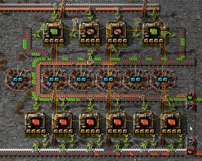
bp = '0eNq1W+1u4zgMfBf/dhaiPiy5r7IoFk7i7hqX2IbtFFcUffeT20OTTeWYnCL/mtYZUpRID4fqa7Y9nOp+aNope3jNml3XjtnDz9dsbH631WH+3fTS19lD1kz1McuztjrOn6pxrI/bQ9P+3hyr3Z+mrTcme8uzpt3X/2YP9JavQjxV47SZhqod+26YNtv6MF0g6LfHPKvbqZma+sOj9w8vv9rTcVsP0cRNoDzruzF+t2tn+xGv8D9cnr1kDxtDP1y0s2+GevfxgJ69vYLXQvhCBm+E8KUM3grhgwzefcKPU7X7Z9O0Yz1M8S9fkD19IquInMAqZK56JXPVC+FJBh8+4Y/1vjkdN/UhPj40u03fHeoEvv4rHvHbdfP7z7Y7DfMhpzI3/jFhphSuwshWQUqIr4X4xD8wbu3AkDA1LxB5zgpz01shvjA5vbBykRPiC0sXFfzNDKubKc1PYSGkIMQXVkIqhQUg0K0CEHKrU/mvhQkahGVMC9+mQViFtTBng7DAaMM+k0GvnUlt2WDn97IOLD8d+mL+im9T+MVthnbjffe/gQjfvJO1j3PctfEk75phd2pm92YGN85f7Yduf4qOPEfrm2P8+TDDR59STnl+wTDCeAbpet3Sendd39fDZldt39MWW2kpdSfc0x2j+FmhlgNfpKBJuNJz2t3voBnNX68VrldICoKTJa6xaEOgC1a/gRceHn4B43tWfLyUaNPVAq7fsyr3NvWqNQFtSL5GKrmSEuDC79CpPk9Jw+JvhSVG2eo8mFRcLAG0b9FvLaVN5pbfMQyRiJVJ6mTxzGXtp7UwPuvk23PmbutqFx+7oW1o8w75WT3Hvq73F2VTJzejgGuPY63Aw/iWhY9nrOPUfluiGgIP36nVHb6ARHbYEdrfM1egUX2CiW/WI2S/FyGLNv3MFThUtGDiF2jTz8T3qGjBxA/rO/y9KudKVAngraBQqJLBxKfVCF2QeCRChUZFAOYKDCpiMPGlb2JhFSocKmIw8Yv1HTbf22FhFgdhlSsCzIV4+MIcDsIq5xXMVDSHqXiC8Q0LXyPK1YIM5uEZleZNZize0qlk7xJMTio5P/EOpnC8tcBTLCa+QELTqxsbYLbGc7aE2SZv5qaQDnohGIFgYsZzVsPEkodvcAUgkUUxKWMzXeqcKNlNB3h4xVwOPLxi4iPDq8WzAw+vmM7CwysmPl+KCrQWjBIeUfGcLeERFRP/G5JUapJnZimNKD3ONzBT5a3FwkyVh+9gnsfDLxAhf+lg4qSX5+xVlo79oZnSvl4UqyvcPHtqDvOXFuYh3WnqT9Ovfmi6IRqPjx3qp/m+1Fd3pBxZWKFJKeHo50wM6Wr0U+2fq3YX+5ZvDn5IScdRZ85xP580PJu8n08GHlDezycrHSXS/X1yUp/s/X0qgOaOWDOM2DXBvRgVSRa5wB9JBT4BU3/ZSKKVwNWCRTRSQJfFjDB0BY6LreEeILV782mYW+k0dyHi37U5s/PlmFuAkHPjIrinWq57WgBsmeuph8lncgfjiUhPQ4kCcFNqOSaCDsKtomkF0D5mhK9vuHFYGhXLLC1R1r9ytCHuSZKkkfRC3HnES47F0rRBL7BzDcA3VrgG4CsrXAOwaMc1AF8+5xqAlTyuAVjKYxowCpXfuAYI1d+4BjSqiHENGFQS4xqwqIzFNeBQHYtroEC1J64Bj4pPXAMBVYS4BkpUEmIasArVhLgGCNVxuAY0qpykDDx+9HnzMPfzP+zy7Lkexo8HAllfau+NL12IHd9/xQERxQ=='

To import it and convert it:

circuits = importBlueprint(bp).convert()

importBlueprint returns a Blueprint object. The convert() method converts the blueprint into a nested group. The outer group contains two inner groups. The first inner group is the factory, and the second is the beacons the factory used.

We are generally only interested in the first inner group (the one with the factory). We can view it using the Group.pprint() methods, which is just a nicer formatted version of repr:

circuits[0].pprint()

Group(mch.AssemblingMachine3(rcp.electronic_circuit, modules=4*itm.productivity_module_3, beacons=1*mch.Beacon(2*itm.speed_module_3, blueprintInfo=...)+1*mch.Beacon(2*itm.speed_module_3, blueprintInfo=...)+1*mch.Beacon(2*itm.speed_module_3, blueprintInfo=...), blueprintInfo=...),
      mch.AssemblingMachine3(rcp.copper_cable, modules=4*itm.productivity_module_3, beacons=1*mch.Beacon(2*itm.speed_module_3, blueprintInfo=...)+1*mch.Beacon(2*itm.speed_module_3, blueprintInfo=...)+1*mch.Beacon(2*itm.speed_module_3, blueprintInfo=...)+1*mch.Beacon(2*itm.speed_module_3, blueprintInfo=...), blueprintInfo=...),
      mch.AssemblingMachine3(rcp.copper_cable, modules=4*itm.productivity_module_3, beacons=1*mch.Beacon(2*itm.speed_module_3, blueprintInfo=...)+1*mch.Beacon(2*itm.speed_module_3, blueprintInfo=...)+1*mch.Beacon(2*itm.speed_module_3, blueprintInfo=...)+1*mch.Beacon(2*itm.speed_module_3, blueprintInfo=...), blueprintInfo=...),
      mch.AssemblingMachine3(rcp.electronic_circuit, modules=4*itm.productivity_module_3, beacons=1*mch.Beacon(2*itm.speed_module_3, blueprintInfo=...)+1*mch.Beacon(2*itm.speed_module_3, blueprintInfo=...)+1*mch.Beacon(2*itm.speed_module_3, blueprintInfo=...), blueprintInfo=...),
      mch.AssemblingMachine3(rcp.advanced_circuit, modules=4*itm.productivity_module_3, beacons=1*mch.Beacon(2*itm.speed_module_3, blueprintInfo=...)+1*mch.Beacon(2*itm.speed_module_3, blueprintInfo=...)+1*mch.Beacon(2*itm.speed_module_3, blueprintInfo=...), blueprintInfo=...),
      mch.AssemblingMachine3(rcp.advanced_circuit, modules=4*itm.productivity_module_3, beacons=1*mch.Beacon(2*itm.speed_module_3, blueprintInfo=...)+1*mch.Beacon(2*itm.speed_module_3, blueprintInfo=...)+1*mch.Beacon(2*itm.speed_module_3, blueprintInfo=...)+1*mch.Beacon(2*itm.speed_module_3, blueprintInfo=...), blueprintInfo=...),
      mch.AssemblingMachine3(rcp.advanced_circuit, modules=4*itm.productivity_module_3, beacons=1*mch.Beacon(2*itm.speed_module_3, blueprintInfo=...)+1*mch.Beacon(2*itm.speed_module_3, blueprintInfo=...)+1*mch.Beacon(2*itm.speed_module_3, blueprintInfo=...)+1*mch.Beacon(2*itm.speed_module_3, blueprintInfo=...), blueprintInfo=...),
      mch.AssemblingMachine3(rcp.advanced_circuit, modules=4*itm.productivity_module_3, beacons=1*mch.Beacon(2*itm.speed_module_3, blueprintInfo=...)+1*mch.Beacon(2*itm.speed_module_3, blueprintInfo=...)+1*mch.Beacon(2*itm.speed_module_3, blueprintInfo=...)+1*mch.Beacon(2*itm.speed_module_3, blueprintInfo=...), blueprintInfo=...),
      mch.AssemblingMachine3(rcp.advanced_circuit, modules=4*itm.productivity_module_3, beacons=1*mch.Beacon(2*itm.speed_module_3, blueprintInfo=...)+1*mch.Beacon(2*itm.speed_module_3, blueprintInfo=...)+1*mch.Beacon(2*itm.speed_module_3, blueprintInfo=...), blueprintInfo=...),
      mch.AssemblingMachine3(rcp.advanced_circuit, modules=4*itm.productivity_module_3, beacons=1*mch.Beacon(2*itm.speed_module_3, blueprintInfo=...)+1*mch.Beacon(2*itm.speed_module_3, blueprintInfo=...), blueprintInfo=...))

As shown above, the output of convert() contains each machine individually converted, and the blueprint info is stored along with the object. In most cases this is more information than we need. We can clean this up by calling Group.simplify() and then Group.sorted():

circuits = circuits[0].simplify().sorted()
circuits.pprint()

Group(2*mch.AssemblingMachine3(rcp.copper_cable, modules=4*itm.productivity_module_3, beacons=4*mch.Beacon(2*itm.speed_module_3)),
      2*mch.AssemblingMachine3(rcp.electronic_circuit, modules=4*itm.productivity_module_3, beacons=3*mch.Beacon(2*itm.speed_module_3)),
      mch.AssemblingMachine3(rcp.advanced_circuit, modules=4*itm.productivity_module_3, beacons=2*mch.Beacon(2*itm.speed_module_3)),
      2*mch.AssemblingMachine3(rcp.advanced_circuit, modules=4*itm.productivity_module_3, beacons=3*mch.Beacon(2*itm.speed_module_3)),
      3*mch.AssemblingMachine3(rcp.advanced_circuit, modules=4*itm.productivity_module_3, beacons=4*mch.Beacon(2*itm.speed_module_3)))

As a shortcut, instead of calling convert() then simplify() and finally sorted() we can instead just use the group() method:

circuits = importBlueprint(bp).group()

If we look at flows of the factory, we will notice that there is not quite enough copper cables, so the rates of the electronic circuits will be slightly too high:

circuits.flows().print()

  advanced_circuit 5.45926/s
  copper_cable! -12.9690/s (47.6/s - 60.5690/s)
  electronic_circuit* 13.1876/s (20.9865/s - 7.79895/s)
  iron_plate -14.9904/s
  copper_plate -17/s
  plastic_bar -7.79895/s
  electricity -30.3197 MW

To fix this, we need to wrap the factory in a box, and give the advanced circuit priority:

circuits = box(circuits, outputs = [itm.electronic_circuit, itm.advanced_circuit@'p1'])
circuits.summary()

Box:
       2x copper_cable: AssemblingMachine3  +240% speed +40% prod. +740% energy +40% pollution
       2x electronic_circuit: AssemblingMachine3  @0.711614  +200% speed +40% prod. +684% energy +40% pollution
       6x advanced_circuit: AssemblingMachine3  +212% speed +40% prod. +701% energy +40% pollution
  Outputs: electronic_circuit 7.13537/s (14.9343/s - 7.79895/s), advanced_circuit 5.45926/s
  Inputs: iron_plate -10.6674/s, copper_plate -17/s, plastic_bar -7.79895/s
  Priorities: itm.advanced_circuit: 1

Being able to wrap the converted blueprint in a box to limit flows is the primary advantage of using of using FactorioCalc to analysis flows of a factory over in game tools such as “Rate Calculator” and “Max Rate Calculator”.

See the Blueprints section in the reference manual for more advanced usages.

Space Age

Factorio has support for most aspects of the Spage Age addon, including full support to quality. To use it simply set the game config 'v2.0-sa' instead of 'v2.0':

To plan your factorio for Space Agse you need to simply set the game config to 'v2.0-sa' instead of 'v2.0' for example:

setGameConfig('v2.0-sa');

Note that calling this function creates a completly new set of symbols. Mixing reference to symbols created before and after this call will likely create unexpected results.

Examples for the rest of this guide will assume that the game config is set to 'v2.0-sa'.

Recipe Productivity

Recipe productivity bonuses are fully supported. You can change the productivity bonus for a particular recipe by modifying config.Gameinfo.recipeProductivityBonus in the config.gameInfo object. Note that config.gameInfo is a ContextVar so you need to call ContextVar.get() to retrieve it first. For example to set the productivity bonus for processing units:

 config.gameInfo.get().recipeProductivityBonus[rcp.processing_unit] = frac('0.5')

Recipe productivity bonuses can also be imported from your current game, see Custom Game Configurations.

Presets

FactorioCalc provides a different set of presets for Space Age.

MP_EARLY_GAME is similar to the same preset in the base game. MP_EARLY_MID_GAME is similar to the MP_LATE_GAME preset for the base game. MP_LATE_GAME will use the best machines available, except that rcp.rocket_fuel, rcp.light_oil_cracking and rcp.heavy_oil_cracking will still use a chemical plant instead of a biochamber. MP_LEGENDARY will use legendary machines with legendary productivity 3 modules when applicable, and legendary quality 3 moduless for the recycler except for scrap recycling which doesn’t use any modules by default.

The sciencePacks presets is also provided and includes all the late game sciences, including the Promethium Science Pack.

Quality

FactorioCalc has full support for quality. For simplicity higher quality versions of items and recipes are distinct objects with the name of the quality as the prefix. For example the higher quality versions of itm.electronic_circuit are: itm.uncommon_electronic_circuit, itm.rare_electronic_circuit, itm.epic_electronic_circuit and itm.legendary_electronic_circuit.

Quality modules are fully supported and will change the recipe to output higher quality items in the correct ratios. The maximum quality outputted can be controlled via config.GameInfo.maxQualityIdx, which is a number between 0 and 4, for example: 0 for no quality, 2 for uncommon and rare, and 4 for all quality levels. It defaults to 4.

To aid in creating quality builds the shortcut property .allQualities can be used to return that item or recipe in all qualties (up to config.GameInfo.maxQualityIdx) as a sequence. When used on a recipe the sequence also supports being called to create a machine for each recipe; for example, rcp.legendary_electronic_circuit.allQualities().

The propery .normalQuality can be used as a shortcut for .allQualities[0]. In addition .quality will return the name of the quality for the current item or recipe and .qualityIdx will return the index.

Examples

As an example of using quality let’s try two methods of late game quality grinding for legendary electronic circuits.

The first method will use legendary quality 3 modules for the electronic circuits:

config.machinePrefs.set(presets.MP_LEGENDARY)
withQuality = box([*~rcp.electronic_circuit.allQualities[0:4](modules=itm.legendary_quality_module_3),
                   ~rcp.legendary_electronic_circuit(),
                   *~rcp.electronic_circuit_recycling.allQualities[0:4]()],
                  inputs = rcp.electronic_circuit.inputs,
                  outputs = [itm.legendary_electronic_circuit@1])
withQuality.summary()

b-legendary-electronic-circuit:
    (3.89x)electronic_circuit: LegendaryElectromagneticPlant  -25% speed +50% prod. +31.0% quality
    (0.658x)uncommon_electronic_circuit: LegendaryElectromagneticPlant  -25% speed +50% prod. +31.0% quality
    (0.290x)rare_electronic_circuit: LegendaryElectromagneticPlant  -25% speed +50% prod. +31.0% quality
    (0.108x)epic_electronic_circuit: LegendaryElectromagneticPlant  -25% speed +50% prod. +31.0% quality
    (0.0704x)legendary_electronic_circuit: LegendaryElectromagneticPlant  -75% speed +175% prod. +400% energy +50% pollution
    (0.943x)electronic_circuit_recycling: LegendaryRecycler  -20% speed +24.8% quality
    (0.541x)uncommon_electronic_circuit_recycling: LegendaryRecycler  -20% speed +24.8% quality
    (0.173x)rare_electronic_circuit_recycling: LegendaryRecycler  -20% speed +24.8% quality
    (0.0650x)epic_electronic_circuit_recycling: LegendaryRecycler  -20% speed +24.8% quality
  Outputs: legendary_electronic_circuit 1/s
  Inputs: iron_plate -23.4788/s (5.67220/s - 29.1510/s), copper_cable -70.4363/s (17.0166/s - 87.4529/s)

(Note that the MP_LEGENDARY preset will use legendary quality 3 modules for all recycling recipes, and legendary productivity 3 modules when possible.)

And the second method will instead use legendary productivity 3 modules for the electronic circuits:

withProd =  box([*~rcp.electronic_circuit.allQualities(beacons = 1*mch.LegendaryBeacon(itm.legendary_speed_module_3)),
                 *~rcp.electronic_circuit_recycling.allQualities[0:4]()],
                inputs = rcp.electronic_circuit.inputs,
                outputs = [itm.legendary_electronic_circuit@1])
withProd.summary()

b-legendary-electronic-circuit:
    (0.450x)electronic_circuit: LegendaryElectromagneticPlant  +550% speed +175% prod. +750% energy +50% pollution
    (0.143x)uncommon_electronic_circuit: LegendaryElectromagneticPlant  +550% speed +175% prod. +750% energy +50% pollution
    (0.0597x)rare_electronic_circuit: LegendaryElectromagneticPlant  +550% speed +175% prod. +750% energy +50% pollution
    (0.0250x)epic_electronic_circuit: LegendaryElectromagneticPlant  +550% speed +175% prod. +750% energy +50% pollution
    (0.00559x)legendary_electronic_circuit: LegendaryElectromagneticPlant  +550% speed +175% prod. +750% energy +50% pollution
    (2.51x)electronic_circuit_recycling: LegendaryRecycler  -20% speed +24.8% quality
    (0.799x)uncommon_electronic_circuit_recycling: LegendaryRecycler  -20% speed +24.8% quality
    (0.334x)rare_electronic_circuit_recycling: LegendaryRecycler  -20% speed +24.8% quality
    (0.139x)epic_electronic_circuit_recycling: LegendaryRecycler  -20% speed +24.8% quality
  Outputs: legendary_electronic_circuit 1/s
  Inputs: iron_plate -14.1348/s (15.1298/s - 29.2647/s), copper_cable -42.4045/s (45.3895/s - 87.7940/s)

Surprisingly, even at just 175% productivity it is better to use productivity instead of quality modules for the electronic circuits. This also requires fewer machines as we can use speed beacons.

It is also possible to try both methods at once at let the solver figure out the optimal combination:

withProd =  box([*~rcp.electronic_circuit.allQualities[0:4](modules=itm.legendary_quality_module_3),
                 *~rcp.electronic_circuit.allQualities(beacons = 1*mch.LegendaryBeacon(itm.legendary_speed_module_3)),
                 *~rcp.electronic_circuit_recycling.allQualities[0:4]()],
                inputs = rcp.electronic_circuit.inputs,
                outputs = [itm.legendary_electronic_circuit@1])
withProd.summary()

b-legendary-electronic-circuit:
    (  0x)electronic_circuit: LegendaryElectromagneticPlant  -25% speed +50% prod. +31.0% quality
    (  0x)uncommon_electronic_circuit: LegendaryElectromagneticPlant  -25% speed +50% prod. +31.0% quality
    (  0x)rare_electronic_circuit: LegendaryElectromagneticPlant  -25% speed +50% prod. +31.0% quality
    (  0x)epic_electronic_circuit: LegendaryElectromagneticPlant  -25% speed +50% prod. +31.0% quality
    (0.450x)electronic_circuit: LegendaryElectromagneticPlant  +550% speed +175% prod. +750% energy +50% pollution
    (0.143x)uncommon_electronic_circuit: LegendaryElectromagneticPlant  +550% speed +175% prod. +750% energy +50% pollution
    (0.0597x)rare_electronic_circuit: LegendaryElectromagneticPlant  +550% speed +175% prod. +750% energy +50% pollution
    (0.0250x)epic_electronic_circuit: LegendaryElectromagneticPlant  +550% speed +175% prod. +750% energy +50% pollution
    (0.00559x)legendary_electronic_circuit: LegendaryElectromagneticPlant  +550% speed +175% prod. +750% energy +50% pollution
    (2.51x)electronic_circuit_recycling: LegendaryRecycler  -20% speed +24.8% quality
    (0.799x)uncommon_electronic_circuit_recycling: LegendaryRecycler  -20% speed +24.8% quality
    (0.334x)rare_electronic_circuit_recycling: LegendaryRecycler  -20% speed +24.8% quality
    (0.139x)epic_electronic_circuit_recycling: LegendaryRecycler  -20% speed +24.8% quality
  Outputs: legendary_electronic_circuit 1/s
  Inputs: iron_plate -14.1348/s (15.1298/s - 29.2647/s), copper_cable -42.4045/s (45.3895/s - 87.7940/s)

Custom Game Configurations

As previous shown, setGameConfig can be used to set or change the game configuration. It can also be used to to load a custom game configuration from a JSON file. Any call to setGameConfig replaces all the symbols in the itm, rcp, mch, and presets packages so any non symbolic references to the old symbols are unlikely to work correctly with the new configuration.

Builtin Game Modes

FactorioCalc supprts the following game modes: v1.1, v1.1-expensive, v2.0, v2.0-sa.

To change the game mode simply call setGameConfig with one of those modes as the first argument, for example for version 1.1 of Factorio:

setGameConfig('v1.1')

Alternative Configurations and Locale Support

FactorioCalc also supports loading a custom game configuration from a JSON file. This is useful as it can include state information from the current game such as if a recipe is enabled and recipe productivity bonus. It is also the only way to get non-English translations for the .descr property and ._find() function.

To load a custom configuration, you first need to export the data from Factorio in the configuration you want. To export the data use the Recipe Exporter mod. Install it, and load a map with the configuration you want. Then, from the console run the dump_recipes command. This command will export the recipes and other needed data to the script-output/recipes.json file. Then, to load the file for the base game use:

setGameConfig('custom', userRecipesFile())

userRecipesFile() assumes Factorio is storing its data in the standard location (%APPDATA%\Factorio for Windows or $HOME/.factorio for Linux). If this is not the case you will need to provide the correct path.

To load a configuration for Space Age instead, change 'custom' to 'custom-sa'.

To skip recipes that have not been researched yet, pass includeDisabled = False into the call to setGameConfig.

When loading a custom configuration recipe productivity bonus are included by default, to not import them pass importBonuses = False into the call to setGameConfig.

Mod Support

For a simple mod that only adds recipes or makes very simple changes, you can load the configuration like you would in the previous section by calling setGameConfig with 'custom' or 'custom-sa' as the first parameter.

Overhaul mods will take a little more work. For basic support you can just call setGameConfig with the 'mod' as the first parameter. Unlike 'custom' this assumes nothing about the games configuration: the presets package will be empty, produce is unlikely to work for recipes with multiple outputs, and although it will be able to derive recipes for rocket launch products the names will be mangled.

Currently FactorioCalc has builtin support for “Space Exploitation”, “Krastorio 2” and “SEK2” (Space Exploration + Krastorio 2). A recipe file is not provided, however, as any provided is likely to out of date and will not match your exact configuration. To enable support use the name as first parameter to setGameConfig. For additional information see the documentation for the mods module.

Adding Additional Mods

To add support for additional mods it is best to look at the source code, in particular the files factoriocalc/import_.py and factoriocalc/mod.py.

Advanced Usage

Unconstrained Flows

In Space Exploration many recipes create byproducts, and other recipes may consume that byproduct, but not as the only ingredient. If both recipes are used in the same factory the net output of the byproduct may be positive or negative. To handle this the byproduct needs to be marked as unconstrained. The unconstrained parameter of the Box constructor is a simple list of flows you want to mark as unconstrained.

Failure to mark a flow as unconstrained may result in a solution that sets all the machines throttles to zero (or in the lesser case just throttles machines unexpectedly). If this happens the unconstrainedHints property may give you hints about what values might need to be marked as unconstrained, but, as of now, it is not comprehensive. If the hints in unconstrainedHints fail, then the best thing to do is reset the throttles back to 1 using resetThrottle() and use internalFlows() to list the internal flows. Then, carefully evaluate the internal flows to determine if any of them need to marked as unconstrained.

Advanced Beacon Usage

In Krastorio 2 you often only need one machine in the late game due to the high speed of the advanced machines and the number of singularity beacons you can surround it by. FactorioCalc provides several tools to help with the calculation of the number of beacons needed.

The first tool is the use of a counter beacon to bring the speed of the machine, with productivity modules, back to one. This will make it easier to determine the number of speed beacons required based on the number of machines reported. To use a counter beacon simply specify the string counter where ever a beacon is expected. The special string will create a FakeBeacon to counter any negative effects of the modules and bring everything back to one. The easiest way to use a counter beacon is to specify the string as part of call to presets.MP_MAX_PROD when setting config.machinePrefs, for example: config.machinePrefs.set(presets.MP_MAX_PROD(beacon='counter'))

The second tool is the useSpeedBeacons function to let FactorioCalc do the calculation for you. The useSpeedBeacons function will add enough speed beacons to reduce the number of machines needed to one.